Critical transitions in a nutshell

In mathematical theory, tipping points are known as catastrophic bifurcations. Although there are several types of catastrophic bifurcations the idea is most easily illustrated by looking at the well-known fold catastrophe (Fig. 1). To understand how this classical case can arise, note that the equilibrium state of a system can respond in different ways to change in conditions such as increase in exploitation pressure or temperature rise (left hand panels). Although some systems respond smoothly (panel a), change can also be relatively sharp around some threshold condition (b). The situation in which critical transitions can occur arises if this equilibrium curve is ‘folded’ (panel c). Then three equilibria can exist for a given condition. If the system is very close to a bifurcation point (e.g. F₂) a tiny change in the condition, may cause a large shift to the lower branch. Also, close to such a bifurcation a perturbation can easily push the system across the boundary between the attraction basins, as illustrated by the stability landscapes in the right hand graph. Thus these bifurcation points are tipping points where runaway change can produce a large transition in response to a tiny perturbation.

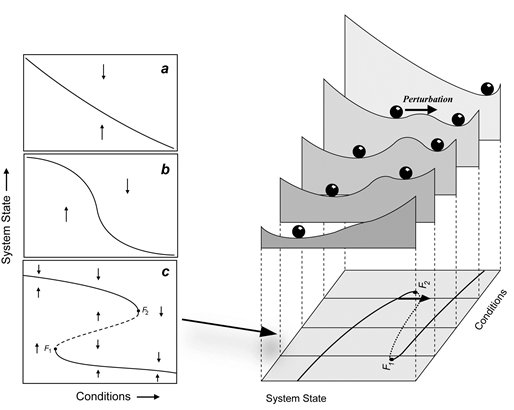
Figure 1 Graphical representation of how critical transitions may happen at tipping points (see text).

We refer to this phenomenon as critical transitions. Although technical details differ depending on the kind of bifurcation, the bottom line is that changing conditions may have seemingly little effect on the state of such systems, until they bring them close to a tipping point. Approaching such a point the basin of attraction around the current state (also referred to a resilience) is shrinking, making the system “brittle” in the sense that a minor perturbation may trigger an overwhelming transition to a contrasting state.